Have you ever wondered why gravity only works in one direction? As an undergraduate physics student, I wondered just that. It started with two equations:

The first is Newton's Law of Gravitation; the second is Coulomb's Law of Electrostatics. Both state that the force F between two objects is proportional to the product of their masses m or charges q, divided by the square of the distance r between them.

Yet while these equations look remarkably similar, there are important differences. First is the minus sign in Newton's equation that is missing from Coulomb's equation. This tells us that two massive bodies attract each other while two similarly charged bodies repel each other.

The second difference is the magnitude of the constants. Coulomb's constant C is a very large number, 8.988 × 10⁹ Nm²/C², implying a strong force. Conversely Newton's constant G is a very small number, 6.670 × 10^-11 Nm²/kg², implying a weak force.

The third difference is that in Coulomb's equation, charge can have both positive and negative values, and the electrostatic force can be either attractive or repulsive. In Newton's equation, though, mass is always positive, and the gravitational force is always attractive.

Why should that be? There's nothing in the math that says mass cannot be negative. Perhaps because we have never encountered negative mass, it has never even occurred to anyone that it might exist. Maybe this third difference is no difference at all—just an unwarranted assumption.

I wondered, if negative mass existed, where would it be? To answer this question, I took some particles—half with positive mass and half with negative mass—threw them together in a computer simulation, and watched where they went. The results were quite remarkable. The like particles tended to clump together and segregate themselves from the unlike particles with both types evolving quickly into all sorts of structures including clusters, filaments, sheets, and large voids. Indeed, it looked exactly like the distribution of galaxies in the large-scale survey maps. A control simulation using only positive mass particles produced a very nice globular cluster demonstrating that both types of matter were necessary to form the kinds of structures seen through the telescope.

So, how do the computer simulations compare to the galactic survey maps? You decide.

---

Results of two simulations. Each used 512 particles, half with positive mass, shown in white, and half with negative mass, shown in red. The only difference was the random initial positions of the particles.

A thin wedge of galaxies mapped by Margaret Geller and John Huchra of the Harvard Smithsonian Center for Astrophycics. The map extends radially to about 150 Mpc (nearly half a billion light-years).

If the computer simulation corresponds to the real Universe, the nearest negative mass would be tens to hundreds of millions of light-years away with the densest concentrations in the middle of the large intergalactic voids.

Detecting negative mass is a more subtle problem. If it exists, it is invisible; else we would have seen it by now. This implies that negative mass does not interact electromagnetically with positive mass and vice versa. However, the theory predicts that it should be detectable by its gravitational effects. A large concentration of mass like a galactic cluster has a gravitational lensing effect on faint blue background galaxies. While a positive mass cluster produces a converging lens, distorting the background galaxies into concentric arcs, negative mass would produce a diverging lens, distorting the background galaxies into radial spokes.

To settle the question, I called a well-known astronomer who had recently published an article on gravitational lensing. After a brief explanation of negative mass, I asked him if he had ever seen background galaxies distorted into spokes in the absence of luminous foreground galaxies. He said he had seen the phenomenon, but he said it was caused by "something else." I asked him what else could cause that, but he refused to answer and abruptly ended the conversation. So until someone can explain to me what that "something else" might be, I consider this prediction to have been proven correct.

Another prediction was that if positive and negative mass exist in equal quantities, the net gravitational mass of the Universe is zero; therefore the deceleration parameter q_o is equal to zero. This was a rather bold prediction since the conventional wisdom was that q_o was equal to one, meaning that the Universe was on the cusp between perpetual expansion and ultimate collapse. With q_o equal to zero, though, not only would the Universe expand forever, it wasn't even slowing down. In fact, when you consider radiation pressure, the expansion would actually be accelerating, albeit very slightly. This bizarre result seemed to doom the theory—that is, until observations later showed that the expansion rate of the Universe was in fact accelerating. Cosmologists are currently reviving Einstein's "cosmological constant" and looking for strange stuff like "dark energy" to explain what negative mass already predicted.

Another perplexing question is our galaxy's motion through the Universe. A slight Doppler shift in the cosmic background radiation indicates that our galaxy, along with thousands of nearby galaxies, is moving in the direction of Perseus at over 630 kilometers per second relative to the rest of the Universe. Many believed we are being pulled along by "The Great Attractor," a huge concentration of mass some 200 million light-years away. The problem with this idea is that when we turn our telescopes in that direction, there is nothing there that could account for this motion. But if there is no Great Attractor, how about a Giant Pusher? One or more large concentrations of negative mass behind us could easily provide the impetus for our observed motion.

Then there is the question of the Big Bang singularity. If all the mass in the observable Universe was once in a tiny volume of space, it would have been "The Mother of All Black Holes." How could anything have escaped from that? Well, if half the mass was negative, the expansion would have been unimpeded by gravity.

A theory must also be compatible with other established theories. So, how do we reconcile negative mass with Newton's Second Law?

When we put negative mass into this equation, the mass is accelerated in the opposite direction of the applied force, which is clearly absurd. We need a slight modification to Newton's Second Law—something I immodestly call the Lucas Generalization:

The absolute value bars do not change the equation except to allow matter to have negative gravitational mass and positive inertial mass. It also makes the two systems symmetrical.

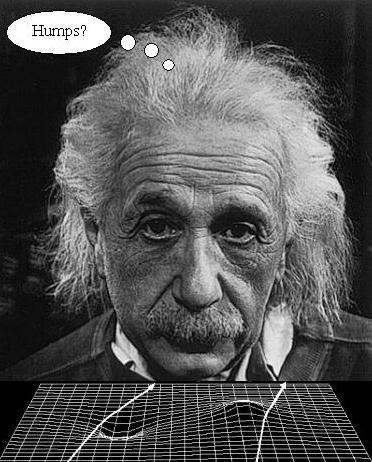
But what about general relativity, which states that gravity is not a force but, rather, curved space-time? The short answer is that negative mass curves space the other way. Consider the familiar "rubber sheet" model of gravity. A massive body produces an indentation so that a ball rolling along the sheet turns towards it. In this model negative mass resides on the other side of the sheet producing humps from which the ball rolls away. However, if we flip the sheet over, it is the negative mass that produces the indentations while the positive mass produces the humps.

Perhaps the best feature of negative mass is that it would not require the wholesale overthrow of our current thinking. The theory appears to be perfectly compatible with the Big Bang, inflation, general relativity, quantum theory, and the Standard Model of particle physics, as well as the latest observations. If it turns out that negative mass does exist, it would solve the problems of large-scale structure and peculiar galactic motion. That would certainly be a matter of some gravity.

About the simulations:

These simulations were run in the spring of 1993 on the fastest computer available in the Southwest Missouri State University Department of Physics and Astronomy -- a brand new 486/DX-33. The machine was located in the faculty workroom, but upperclassmen were allowed to use it during off hours. The simulations each took 60 hours to run, so we would start them late Friday afternoon, and they would finish by early Monday morning.

Each simulation started with 512 particles—half with negative mass and half with positive mass—randomly seeded in a spherical space. The only difference between the two simulations shown here was the random numbers used for the initial positions of the particles. The particles all had equal magnitude of mass and started with zero velocity.

The algorithm simply calculated the acceleration on each particle due to every other particle and applied that acceleration for a fixed length of time (delta t). Since the particles were all the same size, the algorithm was simplified to a single constant divided by the distance r squared. The direction of the acceleration was determined by comparing a single bit representing the positive or negative sign of each particle's mass—similar particles attracted each other, opposite particles repelled each other. After calculating the accelerations for all the particles, each particle was then assigned a new position and velocity vector, and the process was repeated. After every 100 iterations, the computer would write out a data file with the position and velocity of each particle.

The simulations ran through 24,000 iterations generating 240 data files each. We wrote some programs to display the results showing the positive-mass particles in white and the negative-mass particles in red. However, due to the symmetry of the situation, the choice of which particles are labeled positive or negative is completely arbitrary. We could display all the data files in rapid sequence to see the time evolution of the particle clouds, and we could also spin the clouds around a vertical axis so we could see the three-dimensional distribution of the particles. I have converted the output of these programs to AVI video files and made them available here.

In the time evolution videos you will notice a number of high-velocity particles flying out from the main cloud, particularly toward the beginning of the simulation. This is an artifact of the computer algorithm we used. It was caused by using a fixed delta t to calculate the accelerations. When two like particles come close together, they will have a large acceleration and acquire a large velocity sending them shooting off in opposite directions.

We considered different options for dealing with this. One was to decrement delta t when two particles got close so that they would make a smooth orbit around each other. However, since this would have slowed the simulation down considerably, we decided against that. Another option was to make the particles "fuzzy" by using r + b instead of just r in the denominator. By adding a small constant to the distance, it would prevent the denominator from becoming very small and causing a very large acceleration. This, however, would have altered the physics of the problem leaving us open to valid criticism. The third option was to simply let them fly. Once they left the cloud, their effect on the rest of the particles was negligible, and we had enough particles left to get a good result without them. This is the option we chose.

Simulation 1

Sim1.avi  9Mb. This is the time evolution of the first simulation. Download time is about 75 sec. on a 1Mbit broadband connection and about 27 minutes on a 56k dial-up connection.

Sim1Lo.avi  1.25Mb. This is the same as Sim1.avi with a higher compression rate. The quality is only slightly diminished.

Spin1.avi  868Kb. This is the final frame of the first simulation rotating counterclockwise (as viewed from above). This video works best if you set your player to repeat.

Simulation 2

Sim2.avi  9Mb. This is the time evolution of the second simulation.

Sim2Lo.avi  1.3Mb. Same as Sim2 with higher compression.

Spin2.avi  728Kb. This is the final frame of the second simulation rotating counterclockwise (as viewed from above).

Results

In the first simulation, you will notice the formation of three white clusters near the top of the cloud that go on to merge into one larger cluster.

This tends to support the "bottom-up" theory of structure formation. It also tells us that as the Universe ages, it will continue to build larger and larger structures. Also note that the two large white clusters are connected by a thin strand of particles as are the two largest red clusters. This configuration is quite common in the galactic survey maps.

In the second simulation most of the white particles form a single isolated cluster in the center of the cloud while the red particles form a bubble around it. If we were to imagine the red particles as visible galaxies and the white particles as invisible negative-mass galaxies, this would be a perfect example of an intergalactic void or "bubble" as seen in the survey maps.

Remember, the only difference between the two simulations was the random numbers used to assign the initial positions of the particles.